Resolvents of Finite-Dimensional Linear Operators

This topic is something I never learned in linear algebra class. Here I reproduce the exposition by Tosio Kato in Short Introduction to Perturbation Theory for Linear Operators. Go read that book, these notes are just a worse version where I ignore most of the discussions about convergence. But I do fill in some details of the complex integrals and sketch the solutions to some problems, and also include material taken as a given. This is the start of a series of notes.

Definition of the Resolvent

Let $T$$T$ be an linear operator ${\mathbb{C}}^n\to {\mathbb{C}}^n$$\mathbb{C}^n \rightarrow \mathbb{C}^n$. Let the set of eigenvalues of T be $\mathrm{\Sigma }(T)$$\Sigma(T)$. The operator $T-\xi I$$T - \xi I$ is nonsingular whenever $\xi \notin \mathrm{\Sigma }(T)$$\xi \notin \Sigma(T)$, since then $T-\xi \mathbb{I}$$T - \xi \mathbb{I}$ has no zero eigenvalues. In this case we can define $R(\xi )=(T-\xi I{)}^{-1}$$R(\xi) = (T - \xi I)^{-1}$, called the resolvent. The resolvent can refer to both the function $R$$R$ and the operator for any particular value of $\xi$$\xi$.

Properties of $R$$R$

The first resolvent equation is $R({\xi }_1)-R({\xi }_2)=({\xi }_1-{\xi }_2)R({\xi }_1)R({\xi }_2)$$R(\xi_1) - R(\xi_2) = (\xi_1 - \xi_2) R(\xi_1) R(\xi_2)$. This can be seen by the following construction:

The resolvent therefore satisfies the commutation relation $[R({\xi }_1),R({\xi }_2)]=0$$[R(\xi_1), R(\xi_2)] = 0$, since

The Resolvent as a Complex Function

Rearranging the resolvent equation we have

where we have used the Neumann expansion $(I-T{)}^{-1}=\sum _{n=0}^{\mathrm{\infty }}{T}^n$$(I - T)^{-1} = \sum_{n=0}^{\infty} T^n$. So we can expand the resolvent at a given $\xi$$\xi$ in terms of the resolvent somewhere else. The series converges if $({\xi }_2-{\xi }_1)\Vert R({\xi }_1)\Vert <1$$(\xi_2 - \xi_1) \norm{R(\xi_1)} < 1$, and the condition may be weakened. $R(\xi )$$R(\xi)$ is then a holomorphic function.

The other expansion we can use is the Laurent expansion about one of its poles, which are the eigenvalues of $T$$T$. Let $\lambda$$\lambda$ be such an eigenvalue, and for now let it be $0$$0$. The Laurent series is $R(\xi )=\sum _{n=-\mathrm{\infty }}^{n=\mathrm{\infty }}{\xi }^n{A}_n$$R(\xi)= \sum_{n=-\infty}^{n=\infty} \xi^n A_n$ where $A_n$$A_n$ is an operator defined as

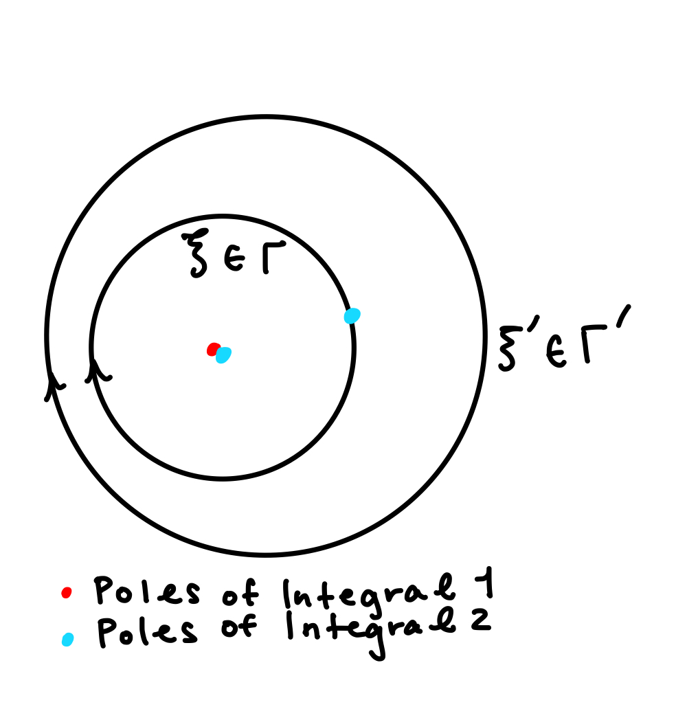
where $\mathrm{\Gamma }$$\Gamma$ is a small clockwise contour enclosing the pole but excluding the other eigenvalues. Let $\mathrm{\Gamma }$$\Gamma$ and ${\mathrm{\Gamma }}^{\prime }$$\Gamma'$ be two contours with ${\mathrm{\Gamma }}^{\prime }$$\Gamma'$ enclosing $\mathrm{\Gamma }$$\Gamma$. Then

The first interior integral must be evaluated keeping in mind that ${\xi }^{\prime }$$\xi'$ will never be equal to $\xi$$\xi$ on the interior of $\mathrm{\Gamma }$$\Gamma$. In this case the singularity comes from ${\xi }^{-n-1}$$\xi^{-n-1}$ and we get

The second interior integral has both poles, so we have

After inserting the integrals we deform the contours back to being the same and rename the variables so they are the same:

So we have recurrence relations for the coefficients of the Laurent expansion. Because we will continue using these operators, we give them special names. Let $P=-A_{-1}$$P=-A_{-1}$, $D=-A_{-2}$$D = -A_{-2}$, and $S=A_0$$S = A_0$. Important cases are:

1. $n=m=-1\Rightarrow A_{-1}{A}_{-1}=-A_{-1}$$n = m = -1 \Rightarrow A_{-1} A_{-1} = - A_{-1}$: So $P=-A_{-1}$$P = -A_{-1}$ is a projection operator.

2. $n,m<0$$n,m < 0$ has $A_{-2}{A}_{-2}=-A_{-3}$$A_{-2} A_{-2} = -A_{-3}$, $A_{-2}{A}_{-3}=-A_{-4}$$A_{-2} A_{-3} = -A_{-4}$, $A_{-2}{A}_{-4}=-A_{-5}$$A_{-2} A_{-4} = -A_{-5}$, etc. Therefore $A_{-k}=-(-A_{-2}^k)=-D^{k-1}$$A_{-k} = -(-A_{-2}^{k}) = -D^{k-1}$ for $k>2$$k > 2$.

3. We also have $A_n=(A_0{)}^{n+1}=S^{n+1}$$A_n = (A_0)^{n+1} = S^{n+1}$ for $n\ge 0$$n \ge 0$.

4. $n=-1,m=-2\Rightarrow A_{-1}{A}_{-2}=A_{-2}{A}_{-1}=-A_{-2}\Rightarrow PD=DP=D$$n=-1, m=-2 \Rightarrow A_{-1} A_{-2} = A_{-2} A_{-1} = -A_{-2} \Rightarrow PD = DP = D$

5. $n=-1,m=0\Rightarrow A_{-1}{A}_0=A_0{A}_{-1}=0\Rightarrow PS=SP=0$$n=-1, m=0 \Rightarrow A_{-1}A_{0} = A_{0}A_{-1} = 0 \Rightarrow PS = SP = 0$

We can break up the Laurent expansion in terms of these special operators:

and shift the pole to wherever the actual eigenvalue $\lambda$$\lambda$ (in the sense that we redo all the work above around the actual eigenvalue) is, and rename our operators ($S\to S_{\lambda }$$S\rightarrow S_\lambda$, etc.) so that we keep track of which eigenvalue we are working with:

In light of 4. and 5. above, we see that

and

So we have decomposed $R(\xi )$$R(\xi)$ into two parts, and accordingly the vector space $\mathcal{X}$$\mathcal{X}$. Let ${\mathcal{M}}_{\lambda }=P_{\lambda }\mathcal{X}$$\mathcal{M}_\lambda = P_\lambda \mathcal{X}$ where $X={\mathbb{C}}^n$$X = \mathbb{C}^n$ and ${\mathcal{M}}_{\lambda }^{\prime }=(1-P_{\lambda })\mathcal{X}$$\mathcal{M}'_{\lambda} = (1 - P_\lambda) \mathcal{X}$, so that $\mathcal{X}={\mathcal{M}}_{\lambda }\oplus {\mathcal{M}}_{\lambda }^{\prime }$$\mathcal{X} = \mathcal{M}_\lambda \oplus \mathcal{M}'_\lambda$.

We now show that $R(\xi )$$R(\xi)$ is a meromorphic function, i.e. none of its singularities are essential. To do this, we examine the convergence of the principal part of the Laurent expansion, i.e. all the negative power terms. We can reproduce them here:

Since we expanded around an isolated singularity, we have no other singularities except at $\lambda$$\lambda$. Therefore $D_{\lambda }$$D_\lambda$ has no other singularities except at $\xi$$\xi$. Since the singularity is right at $\xi$$\xi$, $D_{\lambda }$$D_\lambda$ has a spectral radius of zero, i.e. it has no eigenvalues different from $0$$0$. This implies $D_{\lambda }$$D_\lambda$ is nilpotent. Therefore the principal part only has finitely many terms, and hence converges. So $R(\xi )$$R(\xi)$ is meromorphic.

We can see from the definition of $P_{\lambda }$$P_\lambda$ that

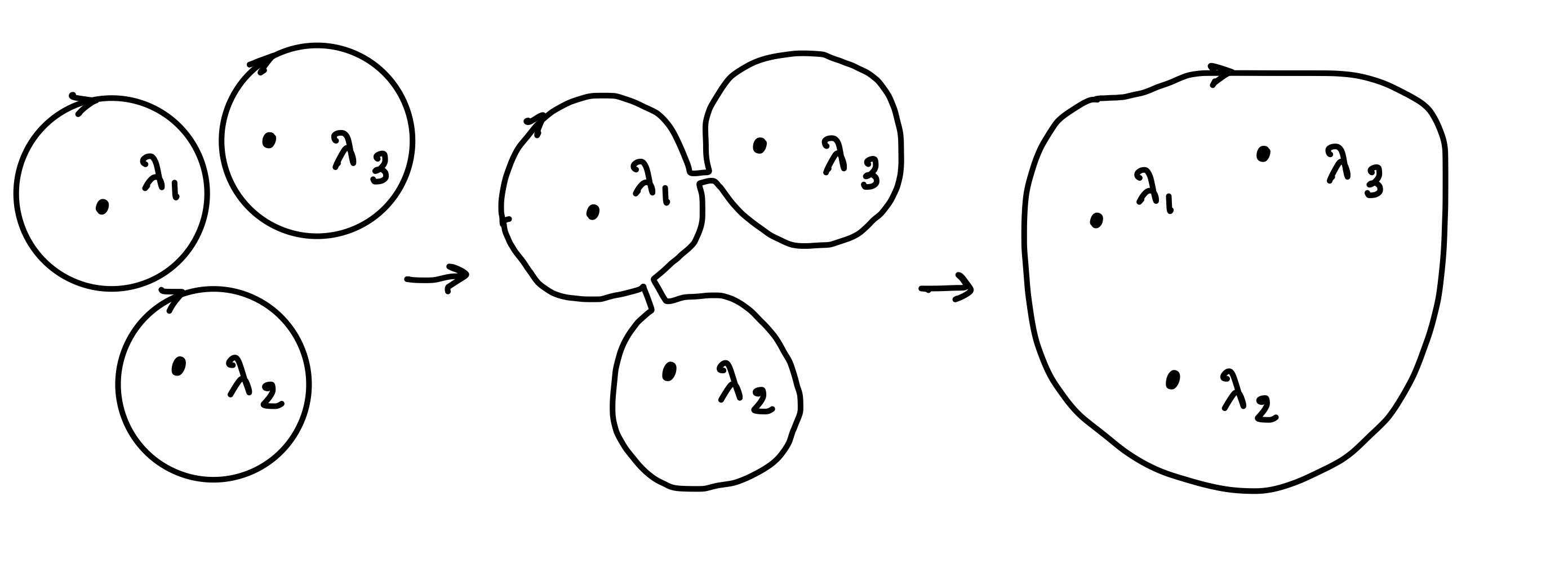
where ${\mathrm{\Gamma }}_{\lambda }$$\Gamma_\lambda$ is a clockwise contour encircling $\lambda$$\lambda$ but passing through no other eigenvalues. Now we can add together the projection operators for different ${\lambda }_k$$\lambda_k$ so that

where we have deformed the contour in each such that the intersection of different countours cancel and we get one contour $\gamma$$\gamma$ going around all the poles ${\lambda }_i$$\lambda_i$.

The meaning of the projection operators becomes clear when we derive the following identities:

1 ) Orthogonality: $P_{\lambda }{P}_{{\lambda }^{\prime }}={\delta }_{\lambda {\lambda }^{\prime }}{P}_{\lambda }$$P_{\lambda} P_{\lambda'} = \delta_{\lambda \lambda'} P_{\lambda}$

Let $\mathrm{\Gamma }$$\Gamma$ and ${\mathrm{\Gamma }}^{\prime }$$\Gamma'$ encircle distinct poles at $\lambda$$\lambda$ and ${\lambda }^{\prime }$$\lambda'$ respectively. Then we the product is zero since the contours encircle no poles:

On the other hand if the poles are the same then by the above relation for the $A_n$$A_n$ we have $P_{\lambda }{P}_{\lambda }=P_{\lambda }$$P_\lambda P_\lambda = P_\lambda$. So we get the above expression.

2 ) Completeness: $\sum P_{\lambda }=I$$\sum P_{\lambda} = I$

Let $\mathrm{\Gamma }$$\Gamma$ be a contour encircling all the eigenvalues. Then we can deform it out to infinity without encountering any further singularities. The behavior of $R(\xi )$$R(\xi)$ at infinity is given by the Neumann expansion

In particular,

So we really can interpret the $P_{\lambda }$$P_\lambda$ as the projection operators onto some space corresponding to $\lambda$$\lambda$. And now noting that $P_{\lambda }$$P_\lambda$ commutes with $T$$T$ because $T$$T$ commutes with $R(\xi )$$R(\xi)$, we can identify it with the eigenspace of $T$$T$ corresponding to $\lambda$$\lambda$.